Expected value versus what actually happened

Expected value tells you what a price is worth on average, and over a single finite run it tells you almost nothing about the specific number you will actually see. That gap between the average and the instance is the entire subject of this post. In Novus Odds you can make the gap visible on demand: configure a synthetic two-outcome market, run a seeded Monte Carlo experiment across as many events as you like, and set the expected value you specified beside the observed ROI the sample really produced. Nothing is wagered and no account is involved. The lab is informational by design, and the point is to measure a relationship, not to chase a result.

What makes the gap tractable is that every assumption is something you name out loud before the run. You set the odds range, the market margin, the pricing uncertainty, the sample size, the stake, and a reproducible seed, then let the engine generate prices, estimate the underlying probabilities, resolve each event, and report the distribution. This article walks through the mechanics in order: what expected value actually claims, how win rate splits by odds bucket, why variance widens the outcome, how streaks and drawdowns surface even under positive expectation, how confidence intervals bound your conclusions, and why favorites and longshots miss their expected value in genuinely opposite ways.

Expected value is the probability-weighted average of every outcome a bet can produce. For a one-unit stake at decimal odds of 3.0 with a true win probability of one in three, a win returns two units and a loss costs one, and the two weighted by their probabilities cancel to zero: a fair price with zero edge. Shift the probability up a little and the EV turns positive; shift the price against you and it turns negative. That number is exact and it is also, crucially, hypothetical. It describes the center of gravity of a distribution you would only ever reach by repeating the event an unlimited number of times.

A finite run is a single draw from the distribution around that center, and there is no rule that says a draw must sit near the middle. The law of large numbers guarantees that observed ROI converges to EV as the number of events grows without bound, but it says nothing reassuring about a thousand events, or ten thousand, especially at long prices. Convergence is a promise about infinity, not about your sample size. This is the mental correction the lab is built to reinforce: read EV as the target the process is aiming at, and read observed ROI as where one particular arrow landed. The distance between them is not an error. It is variance doing exactly what variance does.

A Monte Carlo experiment is only useful if you can trust that its randomness is honest and its results are repeatable, and the seed is what delivers both. When you lock a seed in Novus Odds, the pseudo-random stream that drives price generation and event resolution becomes fixed, so the same configuration produces the same sequence of events every time you run it. That converts a dramatic one-off path into something you can examine like a specimen. You can rerun it, hand the seed to someone else, and know they are looking at the identical experiment rather than a similar-sounding anecdote.

Reproducibility is what lets you isolate cause from noise. The temptation with any simulation is to run it once, see a striking result, and build a story around it. But a single seed produces a single path, and a single path can flatter or damn a price for reasons that have nothing to do with its EV. The disciplined move is to hold the seed, change exactly one knob, and rerun: widen the sample size, shift the odds band, adjust the margin, and watch which change actually moved the outcome. Anything that survives that procedure is a property of the mathematics. Anything that evaporates when you rerun was variance wearing a costume.

A single blended win rate across every price in a run is close to meaningless, because a portfolio that fires on heavy favorites and one that fires on longshots can post the same headline number for completely different reasons. Novus Odds groups results into odds buckets so favorites, moderate underdogs, and longshots are compared on their own terms. Inside each bucket the win rate has a clear reference point: the breakeven probability implied by the price. A -150 favorite implies a sixty percent breakeven, an even-money price implies fifty, and a +900 longshot implies ten. The question is never whether a bucket wins often; it is whether it wins often enough for its price.

Reading win rate against implied probability is what separates a real edge from a comfortable illusion. Favorites win the majority of the time, which feels like success, but that feeling is priced in; a bucket of -150 favorites that hits at fifty-eight percent is losing money despite winning most of its events. Longshots lose the majority of the time, which feels like failure, but a bucket of +900 shots that hits at twelve percent is beating its price. Bucketed win rate strips the emotional charge out of both and replaces it with the only comparison that matters, which is realized frequency against the frequency the odds demand. That is the foundation everything else in the run is built on.

Once buckets exist, the danger is collapsing them back into one number too early. A run can show a slightly positive overall ROI that is entirely manufactured by one lucky longshot bucket, while every other band quietly bled. It can also show a slightly negative overall ROI that conceals a genuinely strong favorite bucket dragged down by longshot noise. Averaging across buckets throws away precisely the information you configured the experiment to expose, because it lets a small number of high-variance events dominate the summary and speak for prices they have nothing to do with.

The lab keeps expected ROI and observed ROI resolved per bucket for exactly this reason. Expected ROI is what the assumptions predict each bucket should return given its prices, probabilities, and the margin you set. Observed ROI is what the sample actually delivered. Placing them side by side, bucket by bucket, turns the run into a diagnostic rather than a verdict. You can see which bands are converging toward their EV and which are still swinging wildly, and you can tell at a glance whether an attractive headline came from a broad, stable effect or from a single windfall that a different seed would erase. The average is a summary; the buckets are the evidence.

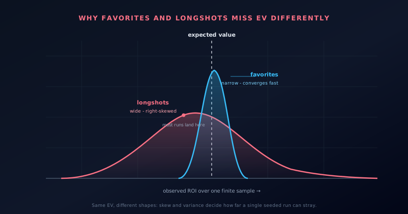
Expected value locates the center of the outcome distribution; variance sets how wide it is, and width is what decides how far a finite run can stray. For a single unit stake, variance rises steeply with the price, because a longshot pays a large multiple on the rare occasions it wins and loses the same single unit every other time. That asymmetry between a big, infrequent payout and a small, frequent loss inflates the spread of possible results. As a rough guide, the per-bet standard deviation grows roughly with the square root of the decimal odds, so a bucket at 10.0 is far noisier per event than a bucket at 1.7, even when both are priced to the same expected value.

The consequence is that variance and sample size trade off directly. Observed ROI stabilizes at a rate governed by the standard error, which shrinks with the square root of the number of events, so quadrupling the sample only halves the noise band. A favorite bucket with low per-bet variance settles down quickly and starts telling the truth about its EV within a manageable run. A longshot bucket with high per-bet variance may still be swinging by tens of percentage points after the same number of events, because each rare win yanks the cumulative line up and each dry spell drags it back down. Variance is not a nuisance layered on top of the result. It is the reason a result needs a sample size at all.

The most important asymmetry in the whole exercise is that favorites and longshots do not just deviate from EV by different amounts, they deviate with different shapes. A favorite payoff distribution is tight and mildly left-skewed: most events return a small profit, a minority return a slightly larger loss, and the many contributing wins pull observed ROI toward EV fast. A longshot payoff distribution is wide and heavily right-skewed: most events lose the stake, and a rare, large win sits far out in a long right tail that carries most of the expected value. Two buckets can share an EV to the decimal and still behave like different animals.

Skew is why the typical finite sample of longshots lands below its EV rather than around it. When most of a distribution's expected value is concentrated in rare large payoffs, a run that happens not to catch enough of those payoffs will understate EV, and that describes the majority of runs; the average is rescued only by the minority that catch a windfall and overstate it dramatically. So the median longshot run underperforms its own expectation while the mean across all runs is correct, and that is not a contradiction, it is what right skew means. Favorites invert the pattern: most runs slightly overstate EV and a rare bad streak understates it. The lab lets you rerun across seeds and watch both tendencies emerge instead of taking them on faith.

Every run produces streaks, and streaks are the single most misread feature of any betting-adjacent process. A bucket with a genuinely positive expected value will still deliver long losing runs, because independent events do not owe you an even spacing of wins. At a ten percent hit rate a losing run of twenty is unremarkable; at forty percent a losing run of eight will happen more often than intuition expects. Novus Odds surfaces the longest losing streak and the deepest drawdown from a peak precisely so you can calibrate against them before mistaking an ordinary cold patch for evidence that the mathematics has changed.

The reason this matters is that a drawdown feels like information and almost never is. Under a fixed EV, the cumulative profit line is a random walk with drift, and even with positive drift the walk can spend long stretches underwater. Seeing that in the lab, where you know the EV was fixed because you set it, inoculates you against the story that a bad run means the edge is gone. The streak and drawdown statistics are not a warning system; they are a description of how rough the ride can be while the underlying expectation is entirely unchanged. Rerun with a new seed and the streaks land in different places while the EV stays exactly where you put it.

A single observed ROI is a point estimate, and a point estimate without a range around it invites overconfidence in both directions. Novus Odds attaches confidence intervals to the cumulative result so the run reports not just what happened but how precisely it pins down the truth. A wide interval says the sample is compatible with a broad set of underlying EVs, which is the honest verdict when the number of events is small or the odds are long. A narrow interval says the sample has genuinely constrained the answer. The width is doing the epistemic work of translating raw outcome into defensible conclusion.

This is where the earlier pieces converge. Interval width is driven by variance and sample size, so the same run length yields a tight interval on a favorite bucket and a loose one on a longshot bucket, mirroring exactly the skew and spread already discussed. An observed ROI that sits above EV but well inside a wide interval is not evidence of an edge; it is noise the interval refuses to rule out. An observed ROI that clears the interval is worth a second look, and the disciplined response is still to rerun under new seeds and larger samples before believing it. The interval is the guardrail that keeps a lucky path from being promoted to a discovery.

The core panel of a run is expected ROI beside observed ROI, and the trap is treating any gap between them as meaningful on its own. A gap is expected; the questions are how large it is relative to the interval, whether it points the same way across seeds, and whether it survives an increase in sample size. If observed trails expected by a few points inside a wide band and flips sign when you reseed, the gap is variance and nothing more. If observed consistently sits on one side of expected across many seeds and the gap holds as the sample grows, then the assumptions you fed the model are producing a systematic effect worth understanding.

The healthiest habit is to interrogate the configuration rather than the outcome. A persistent gap usually traces back to a knob: the margin you set, the pricing uncertainty you allowed, or the odds band you chose, each of which shapes EV before a single event resolves. Because the seed makes runs reproducible, you can attribute the gap to a specific assumption by changing that assumption alone and watching the gap respond. That workflow is the difference between using the lab as a mirror for your own beliefs and using it as an instrument. Expected versus observed is not a scoreboard. It is the readout of a controlled experiment you designed.

How many events you need before observed ROI means anything depends entirely on the bucket, and the lab makes that dependence concrete. Because noise falls with the square root of the sample, and because per-bet variance climbs with the price, the sample size required to pin a longshot bucket to a given precision is dramatically larger than the size required to pin a favorite bucket to the same precision. A favorite band may look settled in a modest run; the same run leaves a longshot band barely started. Increasing the sample size is not a formality you tack on at the end. It is the specific lever that converts a suggestive result into a stable one.

This is why the tool encourages scaling a run up rather than reading too much into a short one. Hold the seed and the configuration, push the event count higher, and watch the observed ROI on each bucket contract toward its expected ROI at a rate that itself tells you something: fast convergence marks a low-variance band you can trust early, slow convergence marks a high-variance band that will keep misleading a small sample. The distribution does not change, only how completely you have sampled it. When someone claims a strategy works or fails from a handful of events, the honest answer is almost always that the sample was too small to distinguish the claim from noise, and the lab is where you can prove it to yourself.

Putting it together, a representative session starts in the Odds Lab, where you configure a synthetic market: pick an odds range spanning favorites through longshots, set a market margin so the prices carry a realistic overround, allow some pricing uncertainty so estimated probabilities wobble, choose a stake, fix a seed, and set a sample size large enough to be worth reading. Generate the outcomes and the engine builds the prices, estimates each event's probability, and resolves the lot. The result is not a single verdict but a distribution, and the analysis view is where the earlier ideas turn into numbers you can point at rather than principles you take on trust.

In the results view you read win rate against implied probability in each bucket, place expected ROI beside observed ROI, and check the interval, the longest losing streak, and the deepest drawdown. Then you do the part that makes it an experiment: reopen the saved run from Experiments, change one knob, and rerun under the same or a new seed to see what actually moved. The Strategy, Sports, Props, Casino, and Datasets labs apply the same loop to different framings, and the Learn route explains the mathematics behind each statistic. Nothing here involves a wager, a deposit, or an account, and results are stored locally in your browser. The output is understanding of how expected value and a finite sample relate, which is the only thing the lab is built to produce.